Microsoft Excel Tips and Tricks

Refer to cell in another worksheet

Reference the worksheet name like this: sheet1!C12

In the example there is a worksheet for each month of the year. To reference a value in cell E7 from the January worksheet in the February worksheet do this:

 =January!E7

Increment month by one

Easy way but not always accurate, just add the number of days to next month:

 =DATE(2009,1,15)+31

Use EDATE from Analysis Toolpak (Tools>Add-ins and check Analysis Toolpak)

 =EDATE(A1,1)

With the Date function

 =DATE(YEAR(A1),MONTH(A1)+1,DAY(A1))

Hide / Unhide Columns

To hide columns just right click on the columns (the letter header at the top) and select hide. But once they are hidden how do you unhide them? Since they are not visible you cannot right click and select unhide.

To unhide column A in the worksheet in Excel versions 97 to 2003

1. Type the cell reference A1 in the Name Box and press the Enter key on the keyboard.
2. Click on the Format menu.
3. Choose Column > Unhide in the menu.
4. Column A will become visible.

To unhide multiple columns in the worksheet - all versions of Excel

For example, you want to unhide columns B, D, and F.

1. In the column header drag select to highlight columns A to G.
2. Right click on the selected columns.
3. Choose Unhide from the menu.
4. The hidden columns and the column letters will be visible.

Even though you can't see the hidden columns as long as you highlight the column before the hidden columns and the column after the hidden columns, then select unhide, you will effectively unhide all of the columns in between.

How Cell Lock and Worksheet Protection Works

By default an Excel worksheet is not protected. Although the state of every cell is locked by default, the locked status is benign unless the worksheet is protected. You must first turn on protection to make the locked state active.

Note: Once the worksheet is protected, you will not be able to change which cells are locked and which cells are unlocked. First, unlock all the cells you wish to be edited before activating protection.

• TO LOCK OR UNLOCK CELLS: Right click on a cell or highlighted area. From the shell menu choose "Format Cells" and click the "Protection" tab.

• TO ACTIVATE WORKSHEET PROTECTION: From the TOOLS menu at the top, choose PROTECTION and enter a simple password.

Editing the locked cells will not be allowed until sheet is unprotected.

AutoSave Add-In

Auto save (autosave) is an add-in feature that is not enabled by default. Goto Tools > Add-Ins & see if "AutoSave Add-In" is listed. If so, check the box to enable autosave.

• Activate AutoSave

To activate the AutoSave feature, follow these steps:

1. On the Tools menu, click Add-Ins.
2. In the Add-Ins dialog box, select the AutoSave Add-in check box, and then click OK.

• Modify AutoSave settings

You can modify AutoSave settings, including how often to save, which workbooks to save, and whether to be prompted before saving.

To modify AutoSave, follow these steps:

1. On the Tools menu, click AutoSave.
2. In the AutoSave dialog box, select the AutoSave options that you want.
3. Click OK.

Microsoft Office 2000 Service Release 1/1a (SR-1/SR-1a) resolves an issue where autosave settings are lost when Excel is reopened. Also an alternative to the autosave addin is something called "AutoSafe" written by Stephen Bullen.

Copying Formulas: Absolute and Relative References

Cell values like =A1 or =A2 increment by 1 when I drag the formula or copy and paste, or fill. Is there some way to lock these values so they don't increment?

• There is indeed. Look up "absolute and relative references" in Help. The short answer is: put a $ before any element you don't want to change. The help will explain the differences among A2, A$2, $A2, and $A$2.

Conditional Formatting: Cell Color

To set the cell color conditional on the value of the cell, use the Excel menu and:

1. Format
2. Conditional Formatting

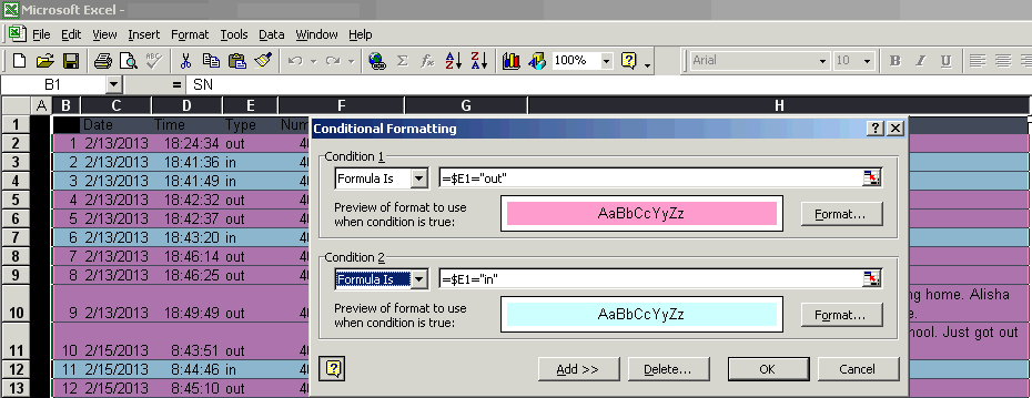
Conditional Formatting: Color Entire Row Based of Value of Text Cell

User asks, "One of the columns I have consists of either "Yes" or "No" text field. I want to have the color of an entire row dependent on the value of a single text field in that row, for the entire excel spreadsheet. Furthermore, this is text data as opposed to numeric field data. So, what I am looking for is to influence the row's color based on the data in one column."

Answer: Select all the columns of rows to be involved. On the toolbar menu goto "Format" then "Conditional Formatting..."; Change condition 1 "Cell Value Is" to "Formula Is"; If the column you want to base your conditional on is column B then use the formula,

=$B1="No"  

And set condition as desired.

source: forum

Partial Text Matching, such as cell contains a text string as part of additional text:

=SEARCH("grocery",F4:F258)

This will match grocery, grocery store, grocery123 or any cell value as long as the string "grocery" is present.

Other conditional operators:

=ISTEXT(A2) 	Checks to see if cell A2 has text (TRUE)
=ISTEXT(A3) 	Checks to see if cell A3 has text (FALSE)
=IF(A2="grocery","OK", "Not OK") 	Checks to see if A2 is grocery (OK)
=IF(A2="lumber", TRUE, FALSE) 	Checks to see if A2 is lumber (FALSE)
=IF(ISNUMBER(SEARCH("v",A2)),"OK", "Not OK") 	Checks to see if A2 contain the letter v (OK)
=ISNUMBER(SEARCH("BD",A3)) 	Checks to see if A3 contains BD (TRUE)

Statistics Based on Spreadsheet Cells

Total number if cells in a column that contain matching text string

• example context: all cells in range of column F that contain string "expenses"

 =COUNTIF(F3:F999,"expenses")

Related

• Microsoft Excel Tips and Tricks
• Microsoft Word Tips and Tricks
• Microsoft Access Tips and Tricks